Inference-Time Scaling for Diffusion/Flow Models
Inference-Time Scaling for Diffusion Models: From Simple Search to Feynman-Kac Steering
Introduction
Diffusion models have revolutionized generative AI, producing impressive results across various domains. However, generating samples with specific desired properties remains challenging. While training-based approaches exist, they require expensive fine-tuning and tie models to specific reward functions. This blog post explores inference-time scaling techniques that can steer diffusion models toward desired outputs without any additional training.
We’ll walk through three increasingly sophisticated approaches:
- Zeroth-order search - searching in the noise space
- Search over paths - searching during the denoising process
- Feynman-Kac steering - a particle-based approach using stochastic dynamics
This implementation demonstrates these concepts on a 2D toy problem, but the same principles apply to the large-scale experiments in “A General Framework for Inference-time Scaling and Steering of Diffusion Models” by Singhal et al., where they show that these methods enable smaller models to outperform larger ones on real tasks like text-to-image generation.
Setup: Imports and Utility Functions
Let’s start by importing necessary libraries and defining utility functions:
# imports and util functions
import torch
import numpy as np
import matplotlib.pyplot as plt
from tqdm import tqdm
from torch import nn, Tensor
from sklearn.datasets import make_moons

device = torch.device('cuda')

def generate_checkerboard_2d(n_samples, square_size=1.0, high_prob=0.8, low_prob=0.2,
                            x_range=(-5, 5), y_range=(-5, 5), max_attempts=None):
    """
    Generate 2D data points from a checkerboard distribution.
    """
    if max_attempts is None: max_attempts = 10 * n_samples

    # Normalize probabilities
    max_prob = max(high_prob, low_prob)

    def checkerboard_density(x, y):
        """Calculate the probability density at point (x, y)"""
        # Determine which square we're in
        square_x = np.floor(x / square_size).astype(int)
        square_y = np.floor(y / square_size).astype(int)

        # Checkerboard pattern: alternating high/low probability
        is_white_square = (square_x + square_y) % 2 == 0

        return np.where(is_white_square, high_prob, low_prob)

    points = []
    attempts = 0

    while len(points) < n_samples and attempts < max_attempts:
        # Generate random candidate points
        batch_size = min(1000, max_attempts - attempts)
        x_candidates = np.random.uniform(x_range[0], x_range[1], batch_size)
        y_candidates = np.random.uniform(y_range[0], y_range[1], batch_size)

        # Calculate densities
        densities = checkerboard_density(x_candidates, y_candidates)

        # Rejection sampling
        accept_probs = np.random.uniform(0, max_prob, batch_size)
        accepted = accept_probs < densities

        # Add accepted points
        for i in np.where(accepted)[0]:
            if len(points) < n_samples:
                points.append([x_candidates[i], y_candidates[i]])

        attempts += batch_size

    return np.array(points)
Flow Model Architecture
We’ll use a simple MLP-based flow model:
class Flow(nn.Module):
    '''Simple MLP flow model'''
    def __init__(self, dim: int = 2, h: int = 64):
        super().__init__()
        self.net = nn.Sequential(
            nn.Linear(dim + 1, h), nn.ELU(),
            nn.Linear(h, h), nn.ELU(),
            nn.Linear(h, h), nn.ELU(),
            nn.Linear(h, dim))

    def forward(self, t: Tensor, x_t: Tensor) -> Tensor:
        return self.net(torch.cat((t, x_t), -1))

    def step(self, x_t: Tensor, t_start: Tensor, t_end: Tensor) -> Tensor:
        '''Using midpoint Euler method'''
        t_start = t_start.view(1, 1).expand(x_t.shape[0], 1)
        return x_t + (t_end - t_start) * self(t=t_start + (t_end - t_start) / 2,
                                             x_t=x_t + self(x_t=x_t, t=t_start) * (t_end - t_start) / 2)
1. Training the Flow Model
We use \(x_0\) as noise, \(x_1\) as data and \(x_t \sim \mathcal{N}(x\mid\alpha_t x_1, \sigma_t^2 I)\).
\(\alpha_t\) and \(\sigma_t\) need to satisfy:
- \[\alpha_1 = \sigma_0 = 1\]
- \[\alpha_0 = \sigma_1 = 0\]
An optimal transport path will be used here, where:
- \[\alpha_t = t\]
- \[\sigma_t = 1-t\]
The flow vector field is then: \(u_t = x_1 - x_0 = \frac{x_1 - x_t}{1 - t}\)
The flow model takes in time \(t\) and noised sample \(x_t\) and predicts the flow vector field \(u_t\)
flow = Flow().to(device)

optimizer = torch.optim.Adam(flow.parameters(), 1e-2)
loss_fn = nn.MSELoss()

for _ in tqdm(range(10000)):
    # Generate data from checkerboard distribution
    x_1 = Tensor(generate_checkerboard_2d(1024*8,
                                          square_size=1.5,
                                          high_prob=1.0,
                                          low_prob=0.0,
                                          x_range=(-3, 3),
                                          y_range=(-3, 3))).to(device)
    x_0 = torch.randn_like(x_1)
    t = torch.rand(len(x_1), 1, device=device)

    # Create interpolated samples
    x_t = (1 - t) * x_0 + t * x_1
    dx_t = x_1 - x_0

    # Train to predict the flow vector field
    optimizer.zero_grad()
    loss_fn(flow(t=t, x_t=x_t), dx_t).backward()
    optimizer.step()
2. Basic Sampling
Once the model approximates the flow vector field \(\frac{dx_t}{dt} = u_t \approx u_t^{\theta}(x_t, t)\), we can start from random noise \(x_0\) and use Euler method to find \(x_1\) iteratively.
\[x_{t+h} = x_{t} + h u_t \approx x_{t} + h u_t^{\theta}(x_t, t)\]x = torch.randn(2048, 2, device=device)
n_steps = 8
fig, axes = plt.subplots(1, n_steps + 1, figsize=(30, 4), sharex=True, sharey=True)
time_steps = torch.linspace(0, 1.0, n_steps + 1, device=device)
axes[0].scatter(x.cpu()[:, 0], x.cpu()[:, 1], s=10)
axes[0].set_title(f't = {time_steps[0]:.2f}')
axes[0].set_xlim(-3.0, 3.0)
axes[0].set_ylim(-3.0, 3.0)
for i in range(n_steps):
with torch.no_grad():
x = flow.step(x_t=x, t_start=time_steps[i], t_end=time_steps[i + 1])
axes[i + 1].scatter(x.cpu()[:, 0], x.cpu()[:, 1], s=10)
axes[i + 1].set_title(f't = {time_steps[i + 1]:.2f}')
plt.tight_layout()
plt.show()

[Figure1: Evolution of samples from noise to data distribution over 8 steps]
3. Inference-Time Scaling
Note that here the model is unconditional and we cannot control the sampling using Euler’s method. However, there are scenarios where one wants to generate certain kind of data, achieving higher scores on some scoring functions. We will explore inference-time scaling with ODE sampler first and then explore inference-time steering toward some scoring functions.
One simple way to do this is to generate a bunch of samples, and select best \(K\) out of those. This is trivially done but can be computationally expensive.
Why Inference-Time Scaling Works
The key insight is that diffusion models define a mapping from noise to data, and by being strategic about:
- Which noise we start from (zeroth-order search)
- How we navigate the denoising path (search over paths)
- When to commit computational resources (FK steering)
We can significantly improve sample quality without any model changes. Think of it as finding better paths through the model’s learned landscape rather than changing the landscape itself.
3.1 Zeroth Order Search
Another way is of similar concept by sampling the neighborhood of noises that generate good samples. Since the model and ODE is deterministic, the sample quality (or scores) is determined by the initial noise. The steps are as follows:
- Given a starting point
pivot\(n\) - Find \(N\) candidates in the pivot’s neighborhood: \(S_n^{\lambda} = \{y: d(y, n) < \lambda\}\) where d is some distance metric
- Run these candidates through ODE and use a verifier/score function to compute the scores
- Find the best candidate, update pivot to be its starting point, and repeat 1-3 for \(n\) cycles.
The scaling complexity is \(N\times n\times steps\).
import functools

def flow_sample(flow, x_start, n_steps=150):
    time_steps = torch.linspace(0, 1.0, n_steps + 1, device=device)
    flow.eval()
    x = x_start.clone()
    with torch.no_grad():
        for i in range(n_steps):
            x = flow.step(x_t=x, t_start=time_steps[i], t_end=time_steps[i + 1])
    return x

def verifier(x_1, target, eps=1e-3):
    '''
    High score for samples close to target point
    '''
    diff = x_1 - target
    return 1.0 / (torch.sum(diff ** 2, dim=-1) + 1e-3)

def line_verifier(x_1, line, tp='horizontal', eps=1e-3):
    '''
    High score for samples close to the line
    '''
    assert tp in ['horizontal', 'vertical']
    x = x_1[:, 1] if tp == 'horizontal' else x_1[:, 0]
    diff = x - line
    return 1.0 / (diff.abs() + 1e-3)

def sample_around_point(center_x, center_y, n_samples, max_distance, device='cpu', dtype=torch.float32):
    """
    Generate n samples uniformly distributed within a circle of radius max_distance
    centered at point A(center_x, center_y).
    """
    # Generate random radii and angles
    # For uniform distribution on disk: r = sqrt(U) * max_radius
    u = torch.rand(n_samples, device=device, dtype=dtype)
    radii = torch.sqrt(u) * max_distance

    # Generate random angles [0, 2π)
    angles = torch.rand(n_samples, device=device, dtype=dtype) * 2 * torch.pi

    # Convert to Cartesian coordinates
    x_offset = radii * torch.cos(angles)
    y_offset = radii * torch.sin(angles)

    # Add to center point
    samples = torch.stack([
        center_x + x_offset,
        center_y + y_offset
    ], dim=1)

    return samples

def sample_around_point_tensor(center_point, n_samples, max_distance):
    """
    Alternative interface that takes center point as a tensor.
    """
    device = center_point.device
    dtype = center_point.dtype

    return sample_around_point(
        center_point[0].item(),
        center_point[1].item(),
        n_samples,
        max_distance,
        device,
        dtype
    )

def inference_time_scaling_zeroth_search(flow, verify_fn, sampling_fn, pivot, cycle=5, n_samples=2048):
    samples, noises = [], []
    pvt = pivot.clone()

    for _ in range(cycle):
        x_start = sampling_fn(pvt, n_samples=n_samples)
        x_final = flow_sample(flow, x_start)
        scores = verify_fn(x_final)
        idx = scores.argmax()
        pvt = x_start[idx]
        samples.append(x_final.cpu())
        noises.append(x_start.cpu())

    return samples, noises

def plot_samples(samples, pivot, target, line=None, tp=None):
    n = len(samples)
    fig, axes = plt.subplots(1, n, figsize=(3*n, 3))
    for i, sample in enumerate(samples):
        axes[i].scatter(sample[:, 0], sample[:, 1], s=2)
        axes[i].set_xlim(-3, 3)
        axes[i].set_ylim(-3, 3)
        axes[i].scatter([pivot[0].item()], [pivot[1].item()], c='black', s=10)
        axes[i].scatter([target[0].item()], [target[1].item()], c='red', s=100, marker='*')
        if line and tp:
            if tp == 'horizontal': axes[i].hlines(line, -3, 3, color='red')
            else: axes[i].vlines(line, -3, 3, color='red')

        axes[i].set_xticks([])
        axes[i].set_yticks([])
    return fig
Now let’s run experiments with different targets:
torch.random.manual_seed(42)
pivot = torch.randn((2, ), device=device)
sampling_fn = functools.partial(sample_around_point_tensor, max_distance=1.0)

## Target at (-2, -2)
target = torch.tensor([-2., -2.], device=device)
verify_fn = functools.partial(verifier, target=target)
samples, noises = inference_time_scaling_zeroth_search(flow, verify_fn, sampling_fn, pivot, cycle=5)
_ = plot_samples(samples, pivot, target)

## Target at (0, 0)
target = torch.tensor([0., 0.], device=device)
verify_fn = functools.partial(verifier, target=target)
samples, noises = inference_time_scaling_zeroth_search(flow, verify_fn, sampling_fn, pivot, cycle=5)
_ = plot_samples(samples, pivot, target)


[Figure2-3: Zeroth-order search results for different target points]
Now let’s try steering towards lines:
torch.random.manual_seed(77)
line1, line2 = torch.randn(2) * 2
line1, line2 = line1.item(), line2.item()
print(line1, line2)
sampling_fn = functools.partial(sample_around_point_tensor, max_distance=1.0)

pivot = torch.tensor([0., 0.], device=device)

## Horizontal line
verify_fn = functools.partial(line_verifier, line=line1, tp='horizontal')
samples, noises = inference_time_scaling_zeroth_search(flow, verify_fn, sampling_fn, pivot, cycle=20)
_ = plot_samples(samples[::4], pivot, target, line=line1, tp='horizontal')

## Vertical line
verify_fn = functools.partial(line_verifier, line=line2, tp='vertical')
samples, noises = inference_time_scaling_zeroth_search(flow, verify_fn, sampling_fn, pivot, cycle=20)
_ = plot_samples(samples[::4], pivot, target, line=line2, tp='vertical')


[Figure4-5: Zeroth-order search results for line targets]
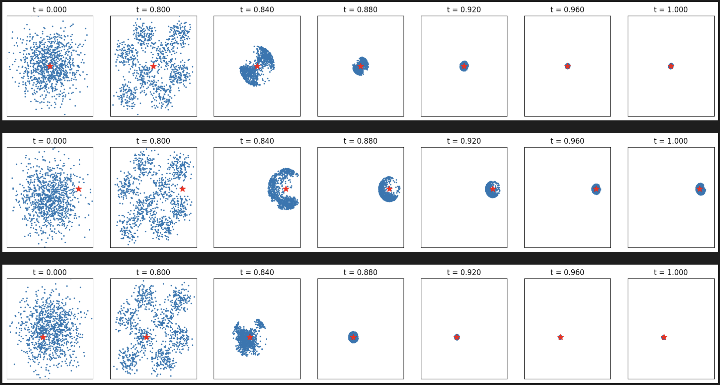
3.2 Search over Paths
Previously, we search over initial noise. We can further do the search during the inference steps \(x_t\) by forward noising \(\Delta f\) for the good samples and then reverse \(\Delta b\). The process is the following:
- Sample \(N\) initial iid noises and run the ODE solver until some time \(t\). The noisy samples \(x_t\) serve as the search starting point.
- Sample \(M\) iid noises for each noisy samples \(x_t\), and simulate the forward noising process from \(t\) to \(t-\Delta f\) to produce \(x_{t-\Delta f}\) with size \(M\).
- Run ODE solver on each \(x_{t-\Delta f}\) to time \(t-\Delta f + \Delta b\), and obtain \(x_{t-\Delta f + \Delta b}\). Run verifiers on these samples and keep the top \(N\) candidates. Repeat steps 2-3 until \(t=1\)
- Run the remaining N samples through random search and keep the best one.
The inference is reversing the noise, and here, we are doing expand -> forward -> reverse -> score -> select
def flow_simulate(flow, x_t, t, t_end, step_size):
    assert t_end > t
    device = x_t.device

    n_steps = int((t_end - t) / step_size)
    time_steps = torch.linspace(t, t_end, n_steps + 1, device=device)
    flow.eval()
    x = x_t.clone()
    with torch.no_grad():
        for i in range(n_steps):
            x = flow.step(x_t=x, t_start=time_steps[i], t_end=time_steps[i + 1])
    return x

def search_over_paths(flow, N, M, t_start, delta_f, delta_b, verify_fn, step_size):
    # delta_f and delta_b are on the time axis
    assert delta_b > delta_f > step_size
    assert N * M > 0
    assert t_start > 0

    flow.eval()
    device = next(flow.parameters()).device

    x_hist = []

    # step 1: Sample N, simulate from 0 to t_start
    x_0 = torch.randn(N, 2, device=device)
    x_t = flow_simulate(flow, x_0, 0.0, t_start, step_size) # (N, 2)

    x_hist.append((0.0, x_0.cpu()))
    x_hist.append((t_start, x_t.cpu()))

    # Step 2-3: Sample M from each x_t, forward to t-df, reverse to t-df+db
    t = t_start
    while t - delta_f + delta_b < 1.0:
        # expand x_t and forward noise
        x_t_df = x_t.repeat((M, 1)) + delta_f * torch.randn((M * N, 2), device=device)

        # reverse to t-df+db
        x_t_df_db = flow_simulate(flow, x_t_df, t - delta_f, t - delta_f + delta_b, step_size)

        # run verifier on noisy samples
        scores = verify_fn(x_t_df_db)

        # pick top N and update x_t and t
        top_idx = torch.argsort(scores, descending=True)[:N]
        x_t = x_t_df_db[top_idx]
        t = t - delta_f + delta_b

        x_hist.append((t, x_t.cpu()))

    # push these N x_t to 1.0
    x_final = flow_simulate(flow, x_t, t, 1.0, step_size)
    x_hist.append((1.0, x_final.cpu()))
    return x_hist

def plot_samples_with_time(samples, target, line=None, tp=None):
    n = len(samples)
    fig, axes = plt.subplots(1, n, figsize=(3*n, 3))
    for i, (t, sample) in enumerate(samples):
        axes[i].scatter(sample[:, 0], sample[:, 1], s=2)
        axes[i].set_xlim(-3, 3)
        axes[i].set_ylim(-3, 3)
        axes[i].scatter([target[0].item()], [target[1].item()], c='red', s=100, marker='*')
        if line and tp:
            if tp == 'horizontal': axes[i].hlines(line, -3, 3, color='red')
            else: axes[i].vlines(line, -3, 3, color='red')
        axes[i].set_xticks([])
        axes[i].set_yticks([])
        axes[i].set_title(f't = {t:.3f}')
    return fig
Let’s run experiments with different targets:
# Target at (0, 0)
target = torch.tensor([0.0, 0.0], device=device)
verify_fn = functools.partial(verifier, target=target)
samples = search_over_paths(flow, 1024, 8, 0.8, 0.1, 0.14, verify_fn, 0.01)
_ = plot_samples_with_time(samples, target)

# Target at (2.0, 0.5)
target = torch.tensor([2.0, 0.5], device=device)
verify_fn = functools.partial(verifier, target=target)
samples = search_over_paths(flow, 1024, 8, 0.8, 0.1, 0.14, verify_fn, 0.01)
_ = plot_samples_with_time(samples, target)

# Target at (-0.5, -0.5)
target = torch.tensor([-0.5, -0.5], device=device)
verify_fn = functools.partial(verifier, target=target)
samples = search_over_paths(flow, 1024, 8, 0.8, 0.1, 0.14, verify_fn, 0.01)
_ = plot_samples_with_time(samples, target)
[Figure6: Search over paths results for different target points]
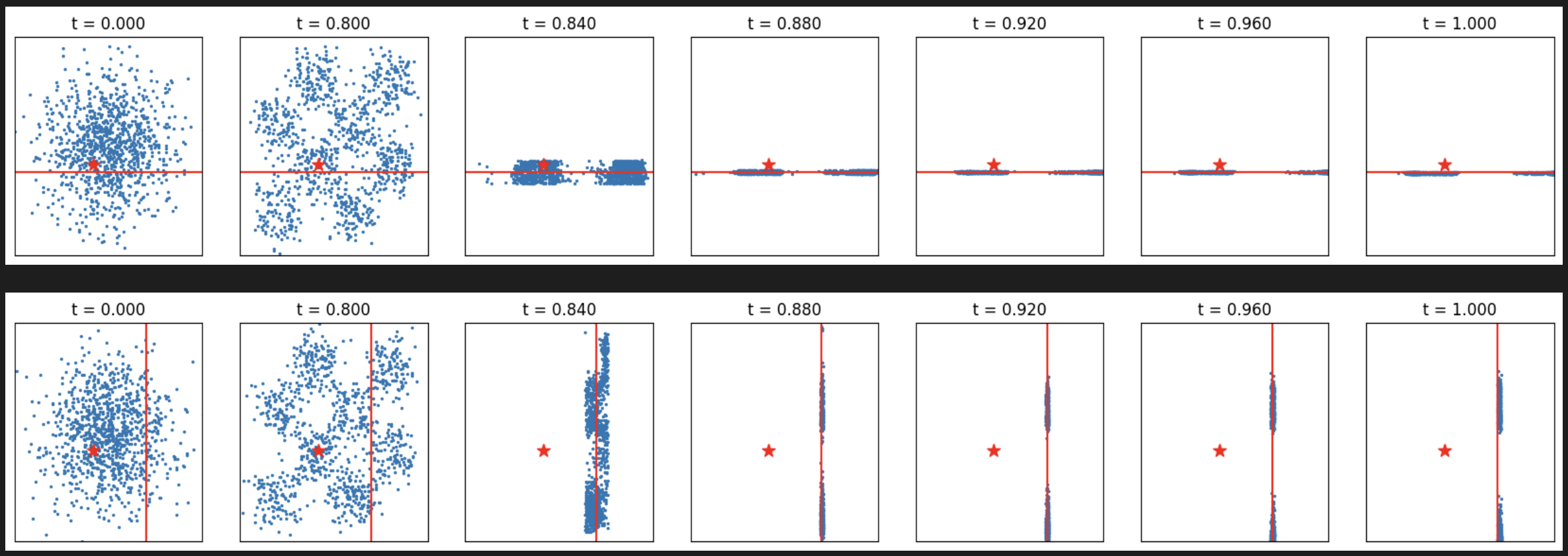
Line targets:
torch.random.manual_seed(77)
line1, line2 = torch.randn(2) * 2
line1, line2 = line1.item(), line2.item()
print(line1, line2)

verify_fn = functools.partial(line_verifier, line=line1, tp='horizontal')
samples = search_over_paths(flow, 1024, 8, 0.8, 0.1, 0.14, verify_fn, 0.01)
_ = plot_samples_with_time(samples, target, line=line1, tp='horizontal')

verify_fn = functools.partial(line_verifier, line=line2, tp='vertical')
samples = search_over_paths(flow, 1024, 8, 0.8, 0.1, 0.14, verify_fn, 0.01)
_ = plot_samples_with_time(samples, target, line=line2, tp='vertical')
[Figure7: Search over paths results for line targets]
3.3 Feynman-Kac Steering
Previously, we looked at ODE sampling. Here, we’ll look into the SDE sampling with Feynman-Kac steering, the most sophisticated approach based on rare-event simulation theory.
Theoretical Foundation
Feynman-Kac (FK) steering is based on Feynman-Kac interacting particle systems (FK-IPS), a rare-event simulation method. The goal is to sample from a tilted distribution:
\[p_{\text{target}}(x_0|c) = \frac{1}{Z} p_\theta(x_0|c) \exp(\lambda r(x_0, c))\]where \(r(x_0, c)\) is a reward function encoding desired properties. FK steering works by:
- Sampling multiple interacting diffusion processes (particles)
- Scoring particles using functions called potentials
- Resampling particles based on their potentials at intermediate steps
The method defines a sequence of distributions \(p_{FK,t}(x_T, x_{T-1}, ..., x_t)\) by tilting the base distribution with potentials \(G_t\):
\[p_{FK,t}(x_T, ..., x_t|c) = \frac{1}{Z_t} p_\theta(x_T, ..., x_t|c) \prod_{s=T}^{t} G_s(x_T, ..., x_s, c)\]The potentials must satisfy: \(\prod_{t=T}^{0} G_t(x_T, ..., x_t, c) = \exp(\lambda r(x_0, c))\)
This ensures that sampling from \(p_{FK,0}\) produces samples from the target tilted distribution.
Intuition: Why Particle-Based Methods Excel
FK steering leverages the power of particle-based methods for rare-event simulation. The key insight is that high-reward samples might be rare under the base model \(p_\theta(x_0)\), but by:
- Running multiple particles in parallel: We explore different regions of the space
- Resampling based on potentials: We focus compute on promising trajectories
- Using intermediate rewards: We can identify good paths early and abandon poor ones
This is fundamentally different from:
- Best-of-N: Which wastes compute on full generation of poor samples
- Gradient guidance: Which is limited to differentiable rewards and can get stuck in local optima
- Fine-tuning: Which permanently changes the model for a single reward
The particle-based approach adaptively allocates computational resources, similar to how evolution explores multiple mutations but only propagates successful ones.
SDE Formulation
The SDE reverse sampling takes the form:
\[dx_t = v(x_t, t)dt - \frac{1}{2}\omega_ts(x_t, t) + \sqrt{\omega_t}dW_t\]where \(v(x_t, t)\) is the flow vector field and \(s(x_t, t) = \nabla\log p_t(x)\) is the score. \(\omega_t\) is some time-dependent diffusion coefficient with \(\omega_1 = 0\). \(dW_t\) is a reverse-time Weiner process.
If \(x_t \sim \mathcal{N}(x\mid\alpha_t x_1, \sigma_t^2 I)\), we have the relationship between flow \(v(x_t, t)\) and score \(s(x_t, t)\):
\[s(x_t, t) = \sigma_t^{-1}\frac{\alpha_tv(x_t, t) - \dot{\alpha_t}x}{\dot{\alpha_t}\sigma_t - \alpha_t\dot{\sigma_t}}\]In the OT case where \(\alpha_t = t\) and \(\sigma_t = 1 - t\):
\[s(x_t, t) = \frac{tv(x_t, t) - x_t}{1-t}\]We can pick \(\omega_t = k\sigma_t = k(1-t)\), which avoids numerical instability when \(t \rightarrow 1\) with \(0<k<1\) controls the stochasticity.
\[dx_t = \left[v(x_t, t) - \frac{k}{2}tv(x_t, t) + \frac{k}{2}x_t \right]dt + \sqrt{k(1-t)}dW_t\]Notice that when \(k=0\), the SDE becomes ODE.
First, let’s implement basic SDE sampling:
def flow_simple_stochastic(flow, x_t, t, t_end, step_size):
    assert t_end > t
    device = x_t.device

    n_steps = int((t_end - t) / step_size)
    time_steps = torch.linspace(t, t_end, n_steps + 1, device=device)
    flow.eval()
    x = x_t.clone()
    x_hist = [x.cpu()]
    with torch.no_grad():
        for i in range(n_steps):
            x = flow.step(x_t=x, t_start=time_steps[i], t_end=time_steps[i + 1])
            x += (time_steps[i + 1] - time_steps[i]) * torch.randn_like(x) * (1.0 - time_steps[i]) ** 0.5
            x_hist.append(x.cpu())
    return x, x_hist

def flow_sde_reverse(flow, x_t, t, t_end, step_size, k=0.1):
    assert t_end > t
    device = x_t.device

    n_steps = int((t_end - t) / step_size)
    time_steps = torch.linspace(t, t_end, n_steps + 1, device=device)
    flow.eval()
    x = x_t.clone()
    x_hist = [x.cpu()]
    with torch.no_grad():
        for i in range(n_steps):
            t1, t2 = time_steps[i], time_steps[i + 1]
            t1 = t1.view(1, 1).expand(x.shape[0], 1)
            v = flow(t=t1 + (t2 - t1) / 2, x_t=x + flow(x_t=x, t=t1) * (t2 - t1) / 2)
            x += (v - 0.5 * k * t1 * v + 0.5 * k * x) * (t2 - t1)
            x += (t2 - t1) * torch.randn_like(x) * (k * (1.0 - t1)) ** 0.5
            x_hist.append(x.cpu())

    return x, x_hist
Compare stochastic vs deterministic sampling:
x_0 = torch.randn((1024, 2), device=device)
_, xhis_1 = flow_simple_stochastic(flow, x_0, 0.0, 1.0, 0.01)
_, xhis_2 = flow_sde_reverse(flow, x_0, 0.0, 1.0, 0.01, k=0.1)

_ = plot_samples(xhis_1[::10], torch.zeros(2), torch.zeros(2))
_ = plot_samples(xhis_2[::10], torch.zeros(2), torch.zeros(2))


[Figure8-9: Comparison of simple stochastic vs SDE reverse sampling]
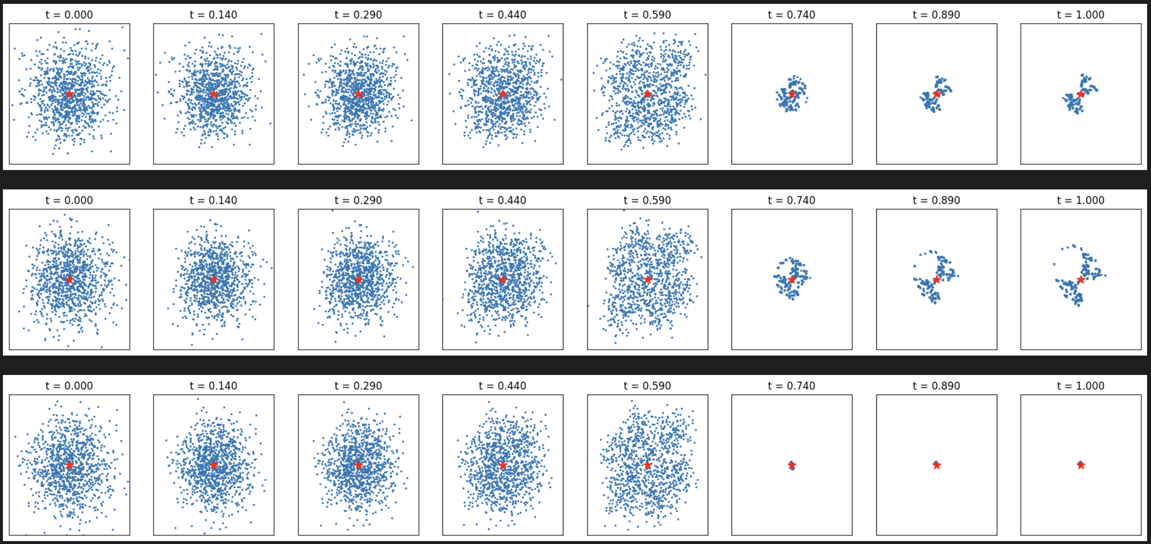
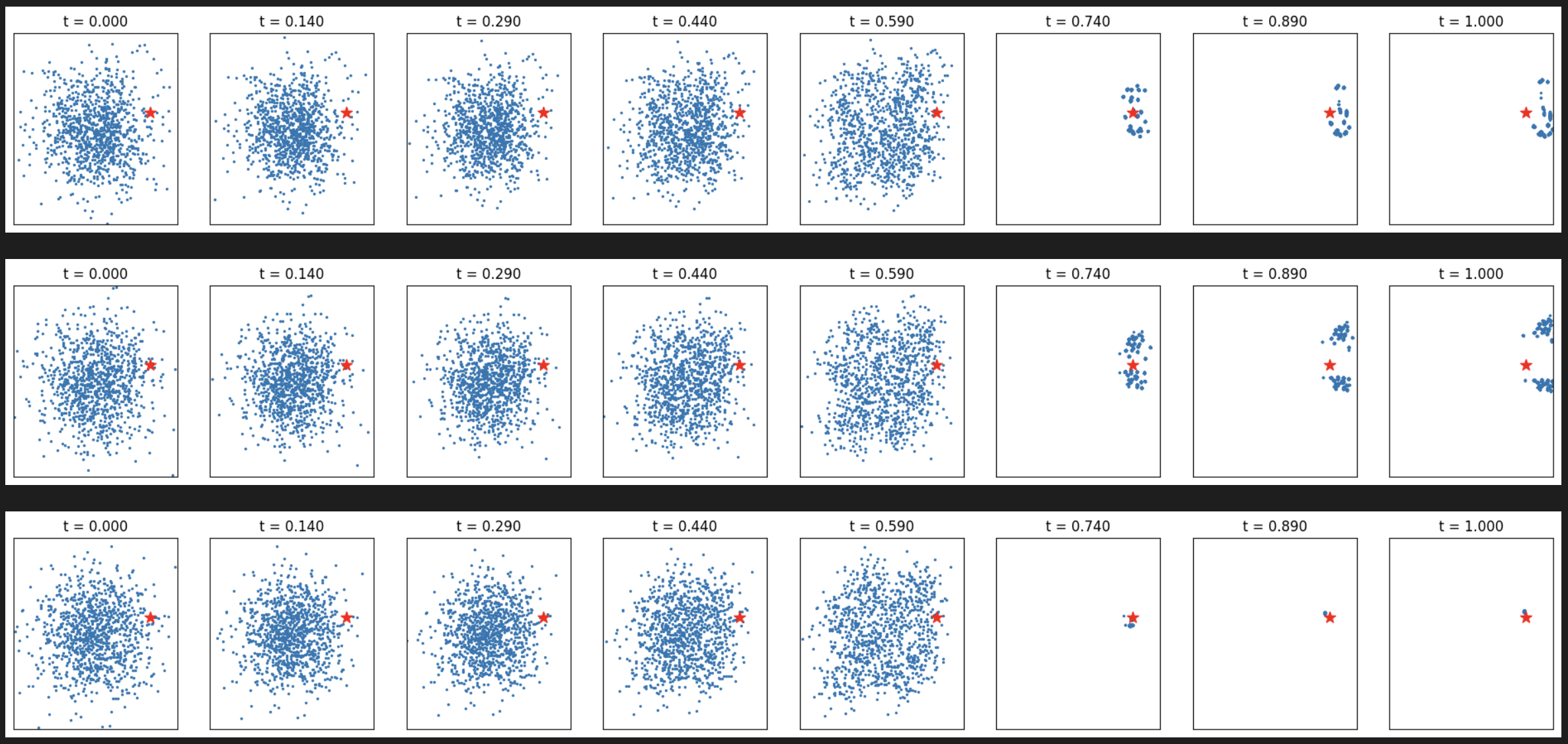
Now the full Feynman-Kac steering implementation:
Potential Functions and Their Roles
FK steering uses different types of potentials that score particles using intermediate rewards \(r_\phi(x_t)\):
- DIFFERENCE: \(G_t(x_t, x_{t+1}) = \exp(\lambda(r_\phi(x_t) - r_\phi(x_{t+1})))\)
- Prefers particles with increasing rewards
- Similar to what Twisted Diffusion Sampler (TDS) uses
- Can assign low scores to particles that reach maximum reward early
- MAX: \(G_t(x_T, ..., x_t) = \exp(\lambda \max_{s=t}^T r_\phi(x_s))\)
- Prefers particles with highest rewards seen so far
- Better for bounded rewards
- May reduce diversity compared to difference potential
- SUM: \(G_t(x_T, ..., x_t) = \exp(\lambda \sum_{s=t}^T r_\phi(x_s))\)
- Selects particles with highest accumulated rewards
- Balances between current and historical performance
def Feyman_Kac_Steering(flow, n_particles,
                        resampling_t_start, resampling_t_end, n_resampling,
                        step_size, reward_fn, potential_tp, lmbda=10.0, k=0.1):

    assert 0 < resampling_t_start < resampling_t_end <= 1.0
    assert potential_tp in ['max', 'add', 'diff']
    device = next(flow.parameters()).device

    # Setup resampling schedule
    n_steps = int(1.0 / step_size)
    time_steps = torch.torch.linspace(0.0, 1.0, n_steps+1, device=device)
    resampling_idx_start = (time_steps - resampling_t_start).abs().argmin().item()
    resampling_idx_end = (time_steps - resampling_t_end).abs().argmin().item()
    resampling_idx_step = int((resampling_idx_end - resampling_idx_start) / n_resampling)
    resampling_idx_step += 1 if resampling_idx_step == 0 else 0
    resampling_idx = list(range(resampling_idx_start, resampling_idx_end, resampling_idx_step))
    print('resampling steps =', len(resampling_idx))

    # init the x and potential
    x_hist = []
    x_t = torch.randn((n_particles, 2), device=device)
    x_hist.append((0.0, x_t.cpu()))
    product_of_potentials, population_rs = torch.ones(n_particles, device=device), torch.zeros(n_particles, device=device)

    for idx, t in enumerate(time_steps):
        if t >= 1.0: break

        # compute score and FK-Resampling
        if idx in resampling_idx:
            rs_candidates = reward_fn(x_t)

            # Compute importance weights based on potential type
            if potential_tp == 'max':
                w = torch.exp(lmbda * torch.max(rs_candidates, population_rs))
            elif potential_tp == 'add':
                rs_candidates = rs_candidates + population_rs
                w = torch.exp(lmbda * rs_candidates)
            elif potential_tp == 'diff':
                diffs = rs_candidates - population_rs
                w = torch.exp(lmbda * diffs)

            w = torch.clamp(w, 0, 1e10)
            w[torch.isnan(w)] = 0.0

            # Resample indices based on weights
            indices = torch.multinomial(w, num_samples=n_particles, replacement=True)
            x_t = x_t[indices]
            population_rs = rs_candidates[indices]

            # Update product of potentials; used for max and add potentials
            product_of_potentials = (product_of_potentials[indices] * w[indices])

        # reverse / propose
        with torch.no_grad():
            tt = t.view(1, 1).expand(x_t.shape[0], 1)
            v = flow(t=tt + step_size / 2, x_t=x_t + flow(x_t=x_t, t=tt) * step_size / 2)
            x_t += (v - 0.5 * k * tt * v + 0.5 * k * x_t) * step_size
            x_t += step_size * torch.randn_like(x_t) * (k * (1.0 - tt)) ** 0.5

        x_hist.append((t.item(), x_t.cpu()))

    # final step
    with torch.no_grad():
        x_t = flow.step(x_t=x_t, t_start=t, t_end=1.0)
    x_hist.append((1.0, x_t.cpu()))

    return x_hist
Now let’s run experiments with different potential types:
# Target at (0, 0)
target = torch.tensor([0.0, 0.0], device=device)
verify_fn = functools.partial(verifier, target=target)

for tp in ['max', 'add', 'diff']:
    print(tp)
    samples = Feyman_Kac_Steering(flow, 1024,
                            resampling_t_start=0.6, resampling_t_end=0.95, n_resampling=5,
                            step_size=0.01, reward_fn=verify_fn, potential_tp=tp)
    _ = plot_samples_with_time(samples[::15]+[samples[-1]], target)
[Figure10: FK steering with different potential types for target (0, 0)]
# Target at (2.0, 0.5)
target = torch.tensor([2.0, 0.5], device=device)
verify_fn = functools.partial(verifier, target=target)

for tp in ['max', 'add', 'diff']:
    print(tp)
    samples = Feyman_Kac_Steering(flow, 1024,
                            resampling_t_start=0.6, resampling_t_end=0.95, n_resampling=5,
                            step_size=0.01, reward_fn=verify_fn, potential_tp=tp)
    _ = plot_samples_with_time(samples[::15]+[samples[-1]], target)
[Figure11: FK steering with different potential types for target (2.0, 0.5)]
# Target at (-0.5, -0.5)
target = torch.tensor([-0.5, -0.5], device=device)
verify_fn = functools.partial(verifier, target=target)

for tp in ['max', 'add', 'diff']:
    print(tp)
    samples = Feyman_Kac_Steering(flow, 1024,
                            resampling_t_start=0.6, resampling_t_end=0.95, n_resampling=5,
                            step_size=0.01, reward_fn=verify_fn, potential_tp=tp)
    _ = plot_samples_with_time(samples[::15]+[samples[-1]], target)
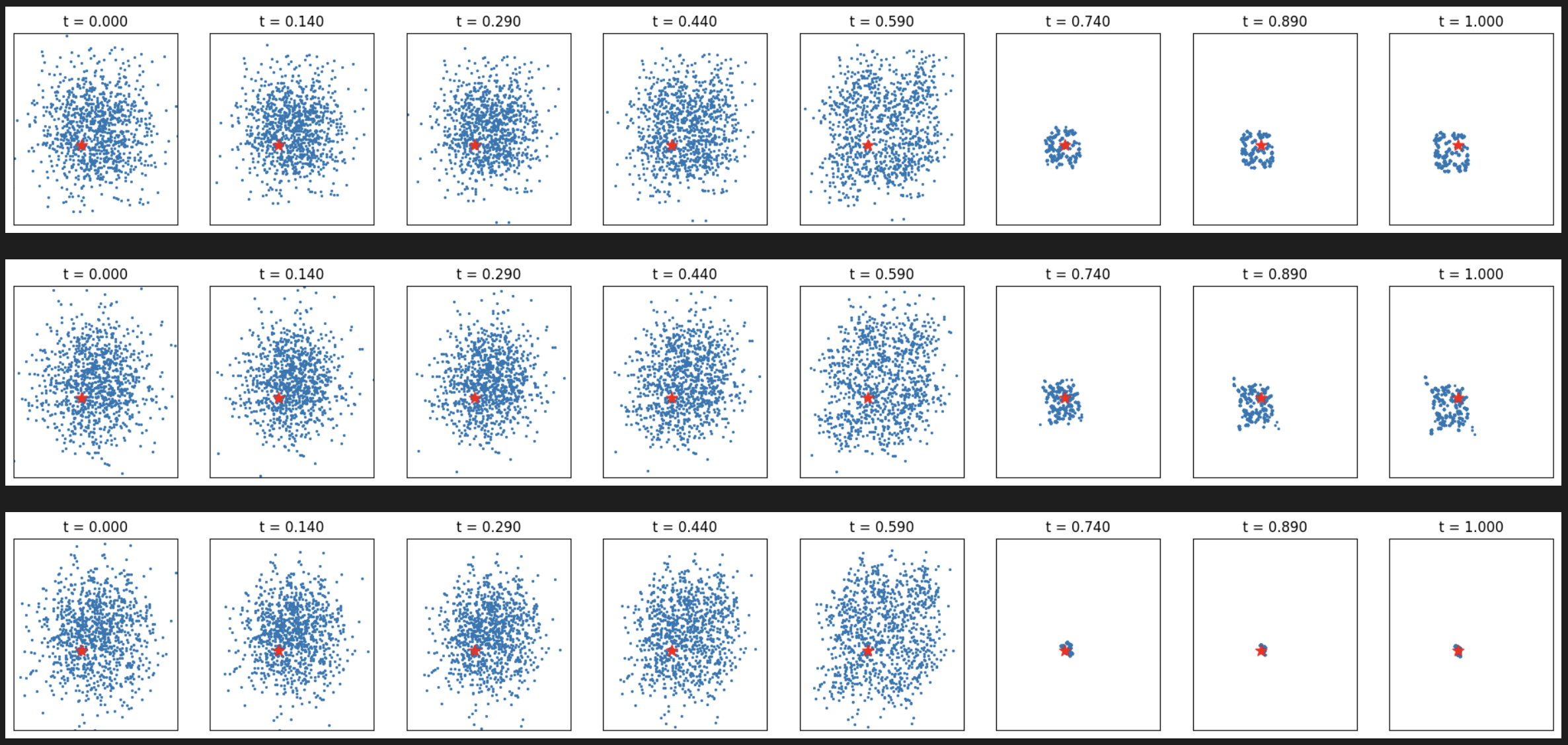
[Figure12: FK steering with different potential types for target (-0.5, -0.5)]
Line targets:
torch.random.manual_seed(77)
line1, line2 = torch.randn(2) * 2
line1, line2 = line1.item(), line2.item()
print(line1, line2)

# Horizontal line
verify_fn = functools.partial(line_verifier, line=line1, tp='horizontal')
for tp in ['max', 'add', 'diff']:
    print(tp)
    samples = Feyman_Kac_Steering(flow, 1024,
                            resampling_t_start=0.6, resampling_t_end=0.95, n_resampling=5,
                            step_size=0.01, reward_fn=verify_fn, potential_tp=tp)
    _ = plot_samples_with_time(samples[::15]+[samples[-1]], target, line=line1, tp='horizontal')

# Vertical line
verify_fn = functools.partial(line_verifier, line=line2, tp='vertical')
for tp in ['max', 'add', 'diff']:
    print(tp)
    samples = Feyman_Kac_Steering(flow, 1024,
                            resampling_t_start=0.6, resampling_t_end=0.95, n_resampling=5,
                            step_size=0.01, reward_fn=verify_fn, potential_tp=tp)
    _ = plot_samples_with_time(samples[::15]+[samples[-1]], target, line=line2, tp='vertical')
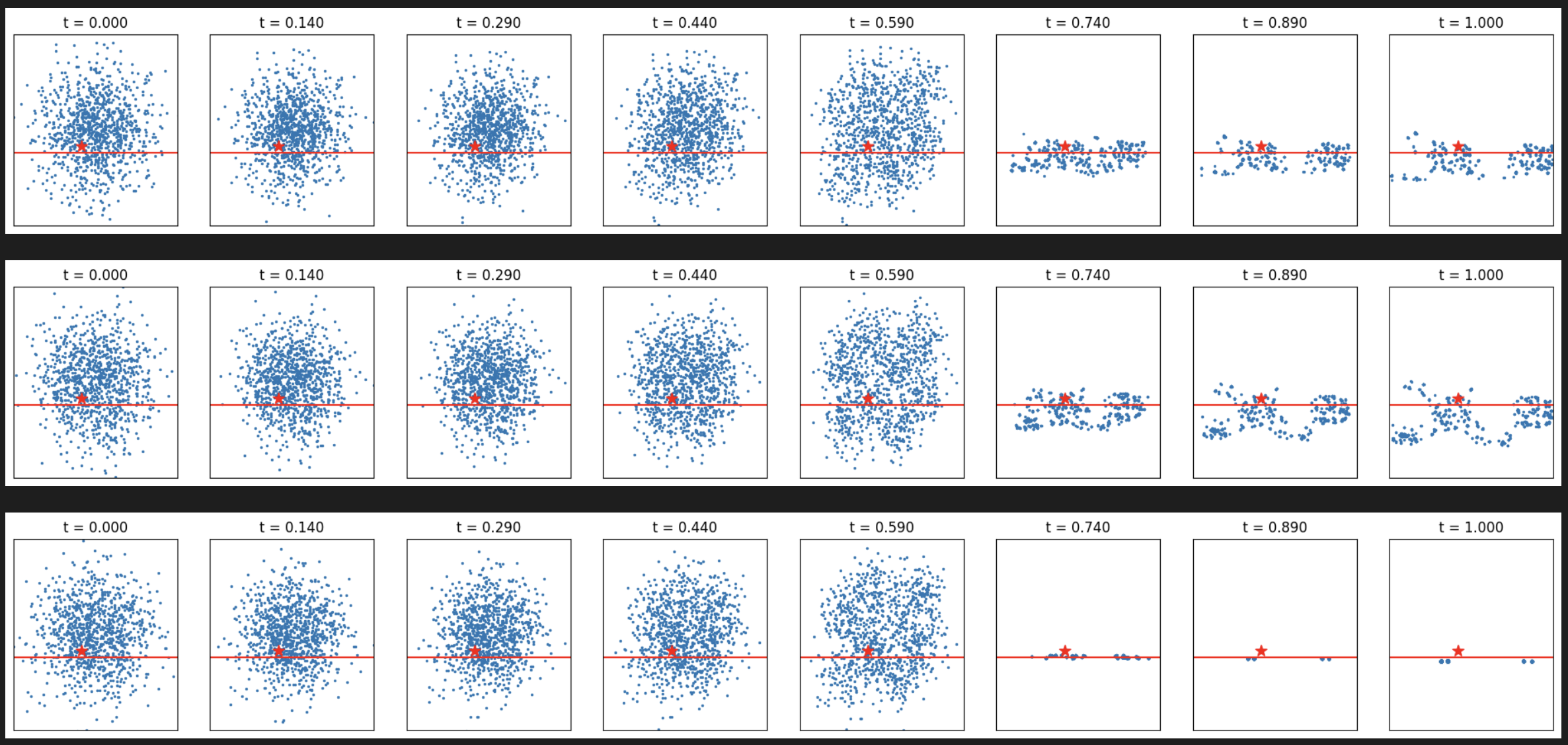
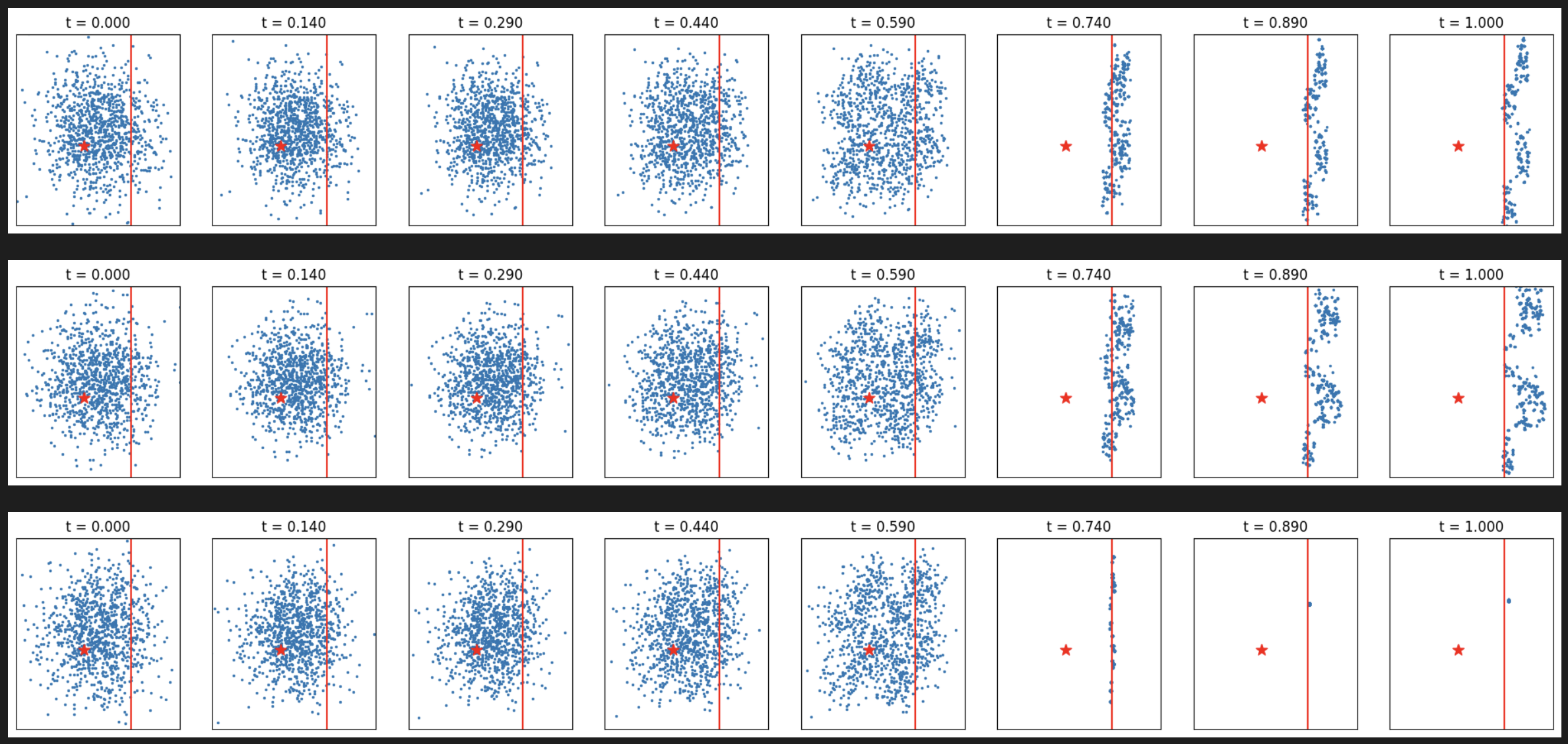
[Figure13-14: FK steering with different potential types for line targets]
Key Insights and Conclusions
Comprehensive Comparison of the Three Approaches
| Method | Search Space | Exploration Strategy | Computational Cost | Key Advantage | Best Use Case |
|---|---|---|---|---|---|
| Zeroth-order | Initial noise only | Local neighborhood search | Low: O(N × n × steps) | Simple to implement | Quick improvements with simple rewards |
| Search over paths | Intermediate states | Branch and prune | Medium: O(N × M × steps) | Dynamic adaptation | Exploring diverse generation paths |
| FK Steering | Full trajectory | Particle resampling with potentials | Medium-High | Principled probabilistic framework | Complex rewards, theoretical guarantees |
Connection to Existing Methods
FK steering provides a unified framework that generalizes several existing approaches:
- Twisted Diffusion Sampler (TDS): Special case using difference potential and gradient guidance
- Soft Value-based Decoding (SVDD): Special case using nested importance sampling
- Best-of-N: Can be seen as FK steering with resampling only at the final step
Practical Considerations
Choosing the Right Method
- Use Zeroth-order search when:
- Computational budget is limited
- Reward function is simple (e.g., distance to target)
- Quick improvements are needed
- Use Search over paths when:
- Need to explore diverse generation paths
- Intermediate states provide useful signal
- Have moderate computational budget
- Use FK Steering when:
- Need principled sampling from complex reward distributions
- Working with bounded rewards (use MAX potential)
- Require theoretical guarantees
- Can afford resampling overhead
Key Takeaways
The success of these methods suggests that inference-time compute may be as valuable as model scale, opening new possibilities for efficient and controllable generation. As the field advances, we may see inference-time scaling become a standard tool alongside model architecture and training data improvements.
Future Directions
- Adaptive particle allocation: Dynamically adjust particles based on task difficulty
- Learned potentials: Train intermediate reward models for better guidance
- Hybrid approaches: Combine FK steering with fine-tuning for further gains
- New applications: Protein design, code generation, and other domains
The Feynman-Kac framework bridges diffusion models with rare-event simulation, providing a principled path toward more controllable and efficient generative AI.