Playing with DDPM | Yen-Lin Chen

The denoising diffusion probabilistic model (DDPM) is the model behind Stable Diffusion, DALL-E 2, Midjourney and Imagen. It has applications in video generation molecular generation, protein generation and superior latent space sampling.

I planned to explore the idea and math behind DDPM and play with some coding and generative image models. I was following the original DDPM paper, this nice paper and this blog for the mathematical formulations and the annotated diffusion model for the implementations.

The Original Diffusion Model

The variance schedule can be improved from linear to cosine
The model can be improved by learning the variances of $p_\theta(x_{t-1} | x_t)$ instead of fixing it
The loss $L = L_{simple} + \lambda L_{vlb}$

The forward process is $p(x_t | x_{t-1})$ and the reverse denoising process is $q(x_{t-1} | x_t)$. A good close-form property is that we don’t need to apply $q$ iteratively to sample $x_t$. We have

\[q(x_t|x_0) = N(x_t; \sqrt{\bar{\alpha}_t}x_0, (1 - \bar{\alpha}_t)I)\] \[\alpha_t = 1 - \beta_t\] \[\bar{\alpha}_t = \prod_{s=1}^t \alpha_s\]

This allows us to optimize random terms of the loss $L$. I.e. randomly sample $t$ during the training to optimize $L_t$

Shown in the Ho et al 2020, one can reparametrize the mean to make the network learn the added noise $\epsilon_\theta(x_t, t)$ for noise level $t$ in the KL terms which constitute the losses. This means that our NN becomes a noise predictor, rather than a direct mean predictor. The mean can be computed as

\[\mu_\theta(x_t, t) = \frac{1}{\sqrt{\alpha_t}}\left( x_t - \frac{\beta_t}{\sqrt{1 - \bar{\alpha}_t}}\epsilon_\theta(x_t, t) \right)\]

The final objective function $L_t$ then looks as the following, for a random time step $t$ given $\epsilon \sim N(0, I)$:

\[|| \epsilon - \epsilon_\theta(x_t, t) ||^2 = || \epsilon - \epsilon_\theta\left( \sqrt{\bar{\alpha}_t}x_0 + \sqrt{1 - \bar{\alpha}_t}\epsilon, t \right)||^2\]

So:

We take a random sample $x_0$ from the real unknown and possibly complex distribution $q(x_0)$
We sample a noise level $t$ uniformly (or complex) between $1$ and $T$ (i.e. random time step)
We sample some noise from a Gaussian distribution and corupt the input by this noise level $t$ using above equations
The neural network is trained to predict this noise based on the corrupted image $x_t$, i.e. noise applied on $x_0$ based on known schedule $\beta_t$
In practice, this is done on batches of data as one uses SGD to optimize the neural network

0. Dependencies

# python: 3.6.9

import os, torch, torchvision, math, requests

import numpy as np
import matplotlib.pyplot as plt
import torch.nn.functional as F

from datetime import datetime
from inspect import isfunction
from functools import partial
from tqdm.auto import tqdm
from einops import rearrange
from PIL import Image
from pathlib import Path
from torch.optim import Adam
from torchvision.utils import save_image
from torch.utils.data import DataLoader
from datasets import load_dataset


# utilities functions
def exists(x): return x is not None

def default(val, d): 
    if exists(val): return val
    return d() if isfunction(d) else d

1. Model Architecture

The model’s input and output have the same dimension. It uses the noisy image at $t$ to predict the corresponding noise and then remove that noise based on variance scheduling to obtain slightly denoised image at $t-1$ and so on until fully denoised at $t=1$. The trick to make the model aware of what kind of filter (lowpass or highpass or something in between) it should behave lies in the time step embedding.

The model consists of 3 parts: UNet, Time Embedding and pixel-pixel Attention.

1.1 Blocks for UNet

# Helper classes
class Residual(torch.nn.Module): 
    
    def __init__(self, fn): 
        super(Residual, self).__init__()
        self.fn = fn
    
    def forward(self, x, *args, **kwargs): 
        return self.fn(x, *args, **kwargs) + x

# up and down sampling from convolution layers
def Upsample(dim): return torch.nn.ConvTranspose2d(dim, dim, 4, 2, 1)
def Downsample(dim): return torch.nn.Conv2d(dim, dim, 4, 2, 1)


# Upsampling
print(Upsample(32))

# Downsampling
print(Downsample(32))

Outputs:

ConvTranspose2d(32, 32, kernel_size=(4, 4), stride=(2, 2), padding=(1, 1))
Conv2d(32, 32, kernel_size=(4, 4), stride=(2, 2), padding=(1, 1))

The UNet blocks using ResNet or ConvNeXT convolutional models:

# GroupNorm
class GNorm(torch.nn.Module): 

    def __init__(self, dim, fn): 
        super(GNorm, self).__init__()
        self.dim = dim
        self.fn = fn
        self.norm = torch.nn.GroupNorm(1, dim)

    def forward(self, x): 
        return self.fn(self.norm(x))

# Block Layer
class Block(torch.nn.Module): 
    
    def __init__(self, dim, output_dim, groups=8): 
        super(Block, self).__init__()
        self.dim = dim
        self.output_dim = output_dim
        self.groups = groups

        # projection, normalize and activation
        self.proj = torch.nn.Conv2d(dim, output_dim, 3, padding=1)
        self.norm = torch.nn.GroupNorm(groups, output_dim)
        self.act = torch.nn.SiLU()

    def forward(self, x, scale_shift=None): 
        x = self.proj(x)
        x = self.norm(x)
        
        if exists(scale_shift): 
            scale, shift = scale_shift
            x = (x * scale) + shift
        
        return self.act(x)

# ResNet: Noise2Noise
class ResNetBlock(torch.nn.Module): 

    def __init__(self, dim, output_dim, *, time_emb_dim=None, groups=8):
        super(ResNetBlock, self).__init__()
        self.dim = dim
        self.output_dim = output_dim
        self.time_emb_dim = time_emb_dim
        self.groups = groups

        self.mlp = torch.nn.Sequential(torch.nn.SiLU(), 
                                       torch.nn.Linear(time_emb_dim, output_dim)) if exists(time_emb_dim) else None

        self.block1 = Block(dim, output_dim, groups=groups)
        self.block2 = Block(output_dim, output_dim, groups=groups)
        self.res_conv = torch.nn.Conv2d(dim, output_dim, 1) if dim != output_dim else torch.nn.Identity()

    def forward(self, x, time_emb=None):
        h = self.block1(x)
        if exists(self.mlp) and exists(time_emb):
            time_emb = self.mlp(time_emb)
            h = rearrange(time_emb, 'b c -> b c 1 1') + h
        
        h = self.block2(h)
        return self.res_conv(x) + h


# ConvNeXT: Noise2Noise

class ConvNextBlock(torch.nn.Module): 
    def __init__(self, dim, output_dim, *, time_emb_dim=None, mult=2, norm=True): 
        super(ConvNextBlock, self).__init__()
        self.dim = dim
        self.output_dim = output_dim
        self.time_emb_dim = time_emb_dim
        
        self.mlp = torch.nn.Sequential(torch.nn.GELU(), torch.nn.Linear(time_emb_dim, dim)) if exists(time_emb_dim) else None
        
        self.ds_conv = torch.nn.Conv2d(dim, dim, 7, padding=3, groups=dim)
        self.net = torch.nn.Sequential(torch.nn.GroupNorm(1, dim) if norm else torch.nn.Identity(), 
                                       torch.nn.Conv2d(dim, output_dim * mult, 3, padding=1), 
                                       torch.nn.GELU(),
                                       torch.nn.GroupNorm(1, output_dim * mult), 
                                       torch.nn.Conv2d(output_dim * mult, output_dim, 3, padding=1))
        self.res_conv = torch.nn.Conv2d(dim, output_dim, 1) if dim != output_dim else torch.nn.Identity()
        
        
    def forward(self, x, time_emb=None): 
        h = self.ds_conv(x)
        
        if exists(self.mlp) and exists(time_emb): 
            time_emb = self.mlp(time_emb)
            h = rearrange(time_emb, 'b c -> b c 1 1')

        h = self.net(h)
        # print(h.shape)
        return self.res_conv(x) + h


# testing the conv blocks
# batch x channel x H x W
bs = 64
batch_image = torch.rand((bs, 3, 44, 44))
print('Batch Image = ', batch_image.shape)
output_dim = 96

TSE = TimeStepEmbedding(32)
batch_t = torch.randint(0, 100, (64, ))
tse = TSE(batch_t)
print('Time Emb = ', tse.shape)

# testing Block
block = Block(3, output_dim)
block_out = block(batch_image)
print('Block output = ', block_out.shape)

# testing ResNetBlock
resnetblock = ResNetBlock(3, output_dim, time_emb_dim=32)
resnetblock_out = resnetblock(batch_image, time_emb=tse)
print('ResnetBlock output = ', resnetblock_out.shape)

# testing ConvNextBlock
convnectblock = ConvNextBlock(3, output_dim, time_emb_dim=32)
convnectblock_out = convnectblock(batch_image, time_emb=tse)
print('ConvnextBlock output = ', convnectblock_out.shape)

Output:

Batch Image =  torch.Size([64, 3, 44, 44])
Time Emb =  torch.Size([64, 32])
Block output =  torch.Size([64, 96, 44, 44])
ResnetBlock output =  torch.Size([64, 96, 44, 44])
ConvnextBlock output =  torch.Size([64, 96, 44, 44])

1.2 Time Embeddings

The time embeddings are from the sequence positional encoding of the Transformer paper.

class TimeStepEmbedding(torch.nn.Module): 

    def __init__(self, dim): 
        super(TimeStepEmbedding, self).__init__()
        assert dim % 2 == 0, 'Dimension has to be even number'
        self.dim = dim

    def forward(self, time): 
        # time is a tensor
        device = time.device
        half_dim = self.dim // 2
        embeddings = math.log(10000) / (half_dim - 1)
        embeddings = torch.exp( -torch.arange(half_dim, device=device) * embeddings)
        embeddings = time[:, None] * embeddings[None, :]
        embeddings = torch.cat([embeddings.sin(), embeddings.cos()], dim=-1)
        return embeddings


# test time embeddings
TSE = TimeStepEmbedding(64)
batch_t = torch.randint(0, 100, (10, ))
print('batched time:', batch_t.shape)

batch_tse = TSE(batch_t)
print('batched time embeddings:', batch_tse.shape)

Output:

batched time: torch.Size([10])
batched time embeddings: torch.Size([10, 64])

1.3 Attention

2 variants of attention:

regular multi-head self-attention (as used in the Transformer),
linear attention variant (Shen et al., 2018), whose time- and memory requirements scale linear in the sequence length, as opposed to quadratic for regular attention.

# Original Attention (in the Conv Net Context)
class Attention(torch.nn.Module): 

    def __init__(self, dim, heads=4, dim_head=32):
        super(Attention, self).__init__()
        self.dim = dim
        self.scale = dim_head ** -0.5
        self.heads = heads

        hidden_dim = dim_head * heads
        self.to_qkv = torch.nn.Conv2d(dim, hidden_dim * 3, 1, bias=False) # compute qkv at the same timne
        self.to_out = torch.nn.Conv2d(hidden_dim, dim, 1)

    def forward(self, x): 
        b, c, h, w = x.shape # batch, channel, height, width
        
        qkv = self.to_qkv(x).chunk(3, dim=1) # (q, k, v) tuple
        q, k, v = map(lambda t: rearrange(t, 'b (h c) x y -> b h c (x y)', h=self.heads), qkv)
        q = q * self.scale

        sim = torch.einsum('b h d i, b h d j -> b h i j', q, k)
        sim = sim - sim.amax(dim=-1, keepdim=True).detach()
        attn = sim.softmax(dim=-1) # batch x heads x (h x w) x (h x w)
        # attention is pixel to pixel weight

        out = torch.einsum('b h i j, b h d j -> b h i d', attn, v)
        out = rearrange(out, 'b h (x y) d -> b (h d) x y', x=h, y=w)

        return self.to_out(out)


# Linear Attention
class LinearAttention(torch.nn.Module):

    def __init__(self, dim, heads=4, dim_head=32):
        super(LinearAttention, self).__init__()
        self.dim = dim
        self.scale = dim_head ** -0.5
        self.heads = heads

        hidden_dim = dim_head * heads
        self.to_qkv = torch.nn.Conv2d(dim, hidden_dim * 3, 1, bias=True)
        self.to_out = torch.nn.Sequential(torch.nn.Conv2d(hidden_dim, dim, 1), 
                                          torch.nn.GroupNorm(1, dim))

    def forward(self, x): 
        b, c, h, w = x.shape
        qkv = self.to_qkv(x).chunk(3, dim=1)
        q, k, v = map(lambda t: rearrange(t, 'b (h c) x y -> b h c (x y)', h=self.heads), qkv)
        
        q = q.softmax(dim=-2)
        k = k.softmax(dim=-2)

        q = q * self.scale
        context = torch.einsum('b h d n, b h e n -> b h d e', k, v)

        out = torch.einsum('b h d e, b h d n -> b h e n', context, q)
        out = rearrange(out, 'b h c (x y) -> b (h c) x y', h=self.heads, y=w)
        return self.to_out(out)

# Test Attention
attn = Attention(96)
attn_out = attn(block_out)
print('Attention out = ', attn_out.shape)


# Test Linear Attention
lattn = LinearAttention(96)
lattn_out = lattn(block_out)
print('Linear Attention out = ', lattn_out.shape)

Output:

Attention out =  torch.Size([64, 96, 44, 44])
Linear Attention out =  torch.Size([64, 96, 44, 44])

1.4 The UNet

The job of the network $\epsilon_\theta(x_t, t)$ is to take in a batch of noisy images + noisy levels and output the noise added to the input. I.e. the network takes a batch of noisy images of shape (batch_size, num_channels, height, width) and batch of noise levels (batch_size, 1) as input. Note that noise levels are just batch_size random integers. And the network returns a tensor of the same shape (batch_size, num_channels, height, width) as the predicted noises.

The network is built up as follows:

First, a conv layer is applied on the batch of noisy images, positional embeddings are computed from the noisy level (an integer).
Second, a sequence of downsampling stahes are applkied. Each downsampling stage consists of
1. 2 ResNet/ConvNeXT blocks
2. Group norm
3. Attention
4. Residual connection
5. Down sampling operation
At the middle of the network, ResNet/ConvNeXT blocks are applied, interleaved with attention
Next, a sequence of upsampling stages are applied
1. 2 ResNet/ConvNeXT blocks
2. Group norm
3. Attention
4. Residual connection
5. Up sampling operation
Finally, a ResNet/ConvNeXT block followed by a conv layer is applied

# # UNet
# # Should use ResNet for the starter

class UNet(torch.nn.Module):
    def __init__(
        self,
        dim,
        init_dim=None,
        out_dim=None,
        dim_mults=(1, 2, 4, 8),
        channels=3,
        with_time_emb=True,
        resnet_block_groups=8,
        use_convnext=True,
        convnext_mult=2,
    ):
        super().__init__()

        # determine dimensions
        self.channels = channels

        init_dim = default(init_dim, dim // 3 * 2)
        self.init_conv = torch.nn.Conv2d(channels, init_dim, 7, padding=3)

        dims = [init_dim, *map(lambda m: dim * m, dim_mults)]
        in_out = list(zip(dims[:-1], dims[1:]))
        # print(in_out)
        
        if use_convnext:
            block_klass = partial(ConvNextBlock, mult=convnext_mult)
        else:
            block_klass = partial(ResNetBlock, groups=resnet_block_groups)

        # time embeddings
        if with_time_emb:
            time_dim = dim * 4
            self.time_mlp = torch.nn.Sequential(
                TimeStepEmbedding(dim),
                torch.nn.Linear(dim, time_dim),
                torch.nn.GELU(),
                torch.nn.Linear(time_dim, time_dim),
            )
        else:
            time_dim = None
            self.time_mlp = None

        # layers
        self.downs = torch.nn.ModuleList([])
        self.ups = torch.nn.ModuleList([])
        num_resolutions = len(in_out)

        for ind, (dim_in, dim_out) in enumerate(in_out):
            is_last = ind >= (num_resolutions - 1)

            self.downs.append(
                torch.nn.ModuleList(
                    [
                        block_klass(dim_in, dim_out, time_emb_dim=time_dim),
                        block_klass(dim_out, dim_out, time_emb_dim=time_dim),
                        Residual(GNorm(dim_out, LinearAttention(dim_out))),
                        Downsample(dim_out) if not is_last else torch.nn.Identity(),
                    ]
                )
            )

        mid_dim = dims[-1]
        self.mid_block1 = block_klass(mid_dim, mid_dim, time_emb_dim=time_dim)
        self.mid_attn = Residual(GNorm(mid_dim, Attention(mid_dim)))
        self.mid_block2 = block_klass(mid_dim, mid_dim, time_emb_dim=time_dim)

        for ind, (dim_in, dim_out) in enumerate(reversed(in_out[1:])):
            is_last = ind >= (num_resolutions - 1)

            self.ups.append(
                torch.nn.ModuleList(
                    [
                        block_klass(dim_out * 2, dim_in, time_emb_dim=time_dim),
                        block_klass(dim_in, dim_in, time_emb_dim=time_dim),
                        Residual(GNorm(dim_in, LinearAttention(dim_in))),
                        Upsample(dim_in) if not is_last else torch.nn.Identity(),
                    ]
                )
            )

        out_dim = default(out_dim, channels)
        self.final_conv = torch.nn.Sequential(
            block_klass(dim, dim), torch.nn.Conv2d(dim, out_dim, 1)
        )

    def forward(self, x, time):
        x = self.init_conv(x)
        t = self.time_mlp(time) if exists(self.time_mlp) else None

        h = []

        # downsample
        for block1, block2, attn, downsample in self.downs:
            x = block1(x, t)
            x = block2(x, t)
            x = attn(x)
            h.append(x)
            x = downsample(x)

        # bottleneck
        x = self.mid_block1(x, t)
        x = self.mid_attn(x)
        x = self.mid_block2(x, t)
        
        # print('mid x: ', x.shape)

        # upsample
        for block1, block2, attn, upsample in self.ups:
            # print('x: ', x.shape, 'h: ', h[-1].shape)
            x = torch.cat((x, h.pop()), dim=1)
            x = block1(x, t)
            x = block2(x, t)
            x = attn(x)
            x = upsample(x)

        return self.final_conv(x)

# Testing the UNet
print('Batch images: ', batch_image.shape)
unet = UNet(32, use_convnext=True)
# Unet with ConvNeXT blocks
# cn_unet = UNet(32, use_convnext=True)
unet_out = unet(torch.randn(64, 3, 128, 128), batch_t)
print(unet_out.shape)
print('Number of Parameters = ', sum(p.numel() for p in unet.parameters() if p.requires_grad))

Output:

Batch images:  torch.Size([64, 3, 44, 44])
torch.Size([64, 3, 128, 128])
Number of Parameters =  14733783

2. Forward Diffusion (Fixed)

Gradually add noises to the imput data (images) in a number ($T$) of steps. Note that this forward process is designed and scheduled but the result of this forward process is stochastic due to the noises.

# linear beta
def linear_beta_schedule(timesteps): 
    beta_start, beta_end = 1e-4, 0.02
    return torch.linspace(beta_start, beta_end, timesteps)

T = 1000

# define betas
betas = linear_beta_schedule(T)

# define alphas
alphas = 1.0 - betas
alphas_cumprod = torch.cumprod(alphas, axis=0)
alphas_cumprod_prev = F.pad(alphas_cumprod[:-1], (1, 0), value=1.0) # shifting alphas_cumprod right
sqrt_recip_alphas = torch.sqrt(1.0 / alphas)

# calculate for diffusion q(x_t | x_{t-1}) and others
sqrt_alphas_cumprod = torch.sqrt(alphas_cumprod)
sqrt_one_minus_alphas_cumprod = torch.sqrt(1.0 - alphas_cumprod)

# calculate for posterior q(x_{t-1} | x_t, t_0)
posterior_variance = betas * (1. - alphas_cumprod_prev) / (1. - alphas_cumprod)

# getting the preset values in the sampling stage
def extract(a, t, x_shape):
    batch_size = t.shape[0]
    out = a.gather(-1, t.cpu())
    return out.reshape(batch_size, *((1,) * (len(x_shape) - 1))).to(t.device)


# Illustrate with Image
url = 'http://images.cocodataset.org/val2017/000000039769.jpg'
image = Image.open(requests.get(url, stream=True).raw)
image

Output:

To standardize the images, we use the following to make images the same size: 128 x 128

# image data processing

from torchvision.transforms import Compose, ToTensor, Lambda, ToPILImage, CenterCrop, Resize

print('Original Image size = ', ToTensor()(image).shape)

image_size = 128

# a series of transformations
transform = Compose([Resize(image_size), 
                     CenterCrop(image_size),
                     ToTensor(), # turn into torch tensor of shape (Height x Width x Channel), divide by 255 in RGB
                     Lambda(lambda t: (t * 2) - 1)])

reverse_transform = Compose([Lambda(lambda t: (t + 1) / 2), 
                             Lambda(lambda t: t.permute(1, 2, 0)), # C x H x W to H x W x C
                             Lambda(lambda t: t * 255.0),
                             Lambda(lambda t: t.numpy().astype(np.uint8)),
                             ToPILImage()])

x_start = transform(image)
print('New Image Size = ', x_start.shape)
x_start = x_start.unsqueeze(0) # adding the batch axis
print('Batched New Image Size = ', x_start.shape)

Output:

Original Image size =  torch.Size([3, 480, 640])
New Image Size =  torch.Size([3, 128, 128])
Batched New Image Size =  torch.Size([1, 3, 128, 128])

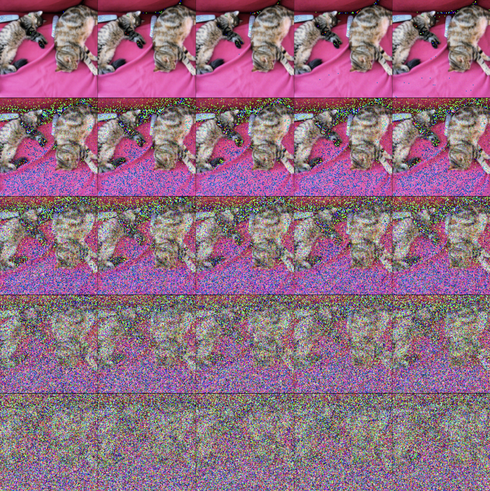
The forward diffusion process of the image is gradually adding noise to the signal until the signal is destroyed.

# sample the time step t given x0
def q_sample(x0, t, noise=None): 
    
    if not exists(noise): noise = torch.randn_like(x0)
    sqrt_alphas_cumprod_t = extract(sqrt_alphas_cumprod, t, x0.shape)
    sqrt_one_minus_alphas_cumprod_t = extract(sqrt_one_minus_alphas_cumprod, t, x0.shape)
    
    return sqrt_alphas_cumprod_t * x0 + sqrt_one_minus_alphas_cumprod_t * noise
    

def get_noisy_image(x0, t): 
    # add noise
    x_noisy = q_sample(x0, t)
    return reverse_transform(x_noisy.squeeze())


# plotting the images from a list
def plot(imgs, with_orig=False, row_title=None, **imshow_kwargs): 
    
    # make 2d even if there is just 1 row
    if not isinstance(imgs[0], list): imgs = [imgs]
    
    num_rows = len(imgs)
    num_cols = len(imgs[0]) + with_orig
    
    fig, axes = plt.subplots(figsize=(200, 200), nrows=num_rows, ncols=num_cols, squeeze=False)
    for row_idx, row in enumerate(imgs): 
        row = [image] + row if with_orig else row
        for col_idx, img in enumerate(row): 
            ax = axes[row_idx, col_idx]
            ax.imshow(np.asarray(img), **imshow_kwargs)
            ax.set(xticklabels=[], yticklabels=[], xticks=[], yticks=[])
    
    if with_orig: 
        axes[0, 0].set(title='Original Image')
        axes[0, 0].title.set_size(8)
    
    if exists(row_title): 
        for row_idx in range(num_rows): 
            axes[row_idx, 0].set(ylabel=row_title[row_idx])
    
    plt.tight_layout()
    
# plot the forward diffusion process
imgs = [[get_noisy_image(x_start, torch.tensor([i + 45 * j])) for i in range(5)] for j in range(5)]
row_title = [45 * j for j in range(45)]
plot(imgs, row_title=row_title)
plt.show()

Output:

3. The Loss Function

The loss function is the L2 or L1 loss between the added noise and the predicted noise. People have found that Huber loss gives better results because it’s less sensitive to outliers in the pixels that might be introduced once in a while by Gaussian.

Note that we train the noise predictor $\epsilon_\theta(x_t, t)$ to achieve this noise-2-noise prediction task

And here, $\epsilon_\theta$ is the UNet.

# This is the loss function 
# Potentially, we have to add more terms, such as KLDiv to the loss function
def p_losses(denoising_model, x0, t, noise=None, loss_type='L1'): 
    
    assert loss_type in ['L1', 'L2', 'huber']
    if not exists(noise): noise = torch.randn_like(x0)
    
    x_noisy = q_sample(x0, t, noise=noise)
    predicted_noise = denoising_model(x_noisy, t)
    
    # print(x_noisy.shape)
    # print(predicted_noise.shape)
    
    if loss_type == 'L1': loss = F.l1_loss(noise, predicted_noise)
    elif loss_type == 'L2': loss = F.mse_loss(noise, predicted_noise)
    elif loss_type == 'huber': loss = F.smooth_l1_loss(noise, predicted_noise)
    else: raise NotADirectoryError()
    
    return loss


# test loss
unet = UNet(32, use_convnext=False)

# batch_size = 64, channel = 3
x0 = torch.randn(64, 3, 64, 64)
# for each batch, tag time to it
ts = torch.randint(0, T, (64, ))
p_losses(unet, x0, ts, loss_type='L1')

Output:

tensor(0.9898, grad_fn=<L1LossBackward0>)

Before Going Too Far..

So now we have a forward diffusion process, a noise-2-noise model and a loss to train the model.

If we have 10 images, T=200 diffusion steps, one epoch needs to go through 2000 images with different noise levels, this number scales with the number of images ….

In training, typically this is a batch b:

t0, img3 | t0
t1, img1 | t1
t2, img9 | t2
t3, img1 | t3

…

tb, img8 | tb

So different from supervised label prediction, the model needs to be trained using a large number of epochs.

4. Data and Datalaoder for diffusion

I used the flower dataset for playing with the DDPM model.

dataset = load_dataset('huggan/flowers-102-categories')
print(len(dataset['train']))
imgs = [dataset['train'][i.item()]['image'] for i in torch.randint(0, 8189, (10, ))]
# imgs = [i.item() for i in torch.randint(0, 8189, (10, ))]
plot(imgs)

Output:

Still, they are of different sizes and need to be standardized:

IMAGE_SIZE = 128
BATCH_SIZE = 64
CHANNELS = 3

flower_transformation = Compose([
    Resize(IMAGE_SIZE),
    CenterCrop(IMAGE_SIZE),
    ToTensor(), # turn into Numpy array of shape HWC, divide by 255
    Lambda(lambda t: (t * 2) - 1),
    
])

flower_reverse_transformation = Compose([
     Lambda(lambda t: (t + 1) / 2),
     Lambda(lambda t: t.permute(1, 2, 0)), # CHW to HWC
     Lambda(lambda t: t * 255.),
     Lambda(lambda t: t.numpy().astype(np.uint8)),
     ToPILImage(),
])

x_start = dataset['train'][999]['image']
x_start = flower_transformation(x_start).unsqueeze(0)
print(x_start.shape)

flower_reverse_transformation(x_start.squeeze(0))

def collate_fn(examples):
    return torch.stack([flower_transformation(example['image']) for example in examples])


dataloader = DataLoader(dataset['train'], collate_fn=collate_fn, batch_size=BATCH_SIZE)
print('dataloader length = ', len(dataloader))

x_start = next(iter(dataloader))
print(x_start.shape)
print()
flower_reverse_transformation(x_start[2, :, :, :])

# transformed_dataset = dataset.with_transform(flower_transformation)

Output:

torch.Size([1, 3, 128, 128])
dataloader length =  128
torch.Size([64, 3, 128, 128])

5. Sampling (Generating)

The sampling is to get a batch of images and time batch. The sampling can be done with no_grad() for speeding up.

@torch.no_grad()
def p_sample(model, x, t, t_index): 
    
    betas_t = extract(betas, t, x.shape)
    sqrt_one_minus_alphas_cumprod_t = extract(sqrt_one_minus_alphas_cumprod, t, x.shape)
    sqrt_recip_alphas_t = extract(sqrt_recip_alphas, t, x.shape)
    
    # Equation 11 in Ho et al. 2020
    # Use the noise-2-noise model to predict the mean
    model_mean = sqrt_recip_alphas_t * (x - betas_t * model(x, t) / sqrt_one_minus_alphas_cumprod_t)
    
    if t_index == 0: return model_mean
    else: 
        posterior_variance_t = extract(posterior_variance, t, x.shape)
        noise = torch.randn_like(x)
        return model_mean + torch.sqrt(posterior_variance_t) * noise
    

@torch.no_grad()
def p_sample_loop(model, shape): 
    
    device = next(model.parameters()).device
    
    b = shape[0]
    
    # start with pure noise (for each example in the batch)
    img = torch.randn(shape, device=device)
    imgs = []
    
    for i in tqdm(reversed(range(0, T)), desc='Sampling Loop Timestep', total=T):
        img = p_sample(model, img, torch.full((b, ), i, device=device, dtype=torch.long), i)
        imgs.append(img.cpu().numpy())
    
    return imgs

@torch.no_grad()
def sample(model, image_size=IMAGE_SIZE, batch_size=BATCH_SIZE, channels=CHANNELS): 
    return p_sample_loop(model, shape=(batch_size, channels, image_size, image_size))

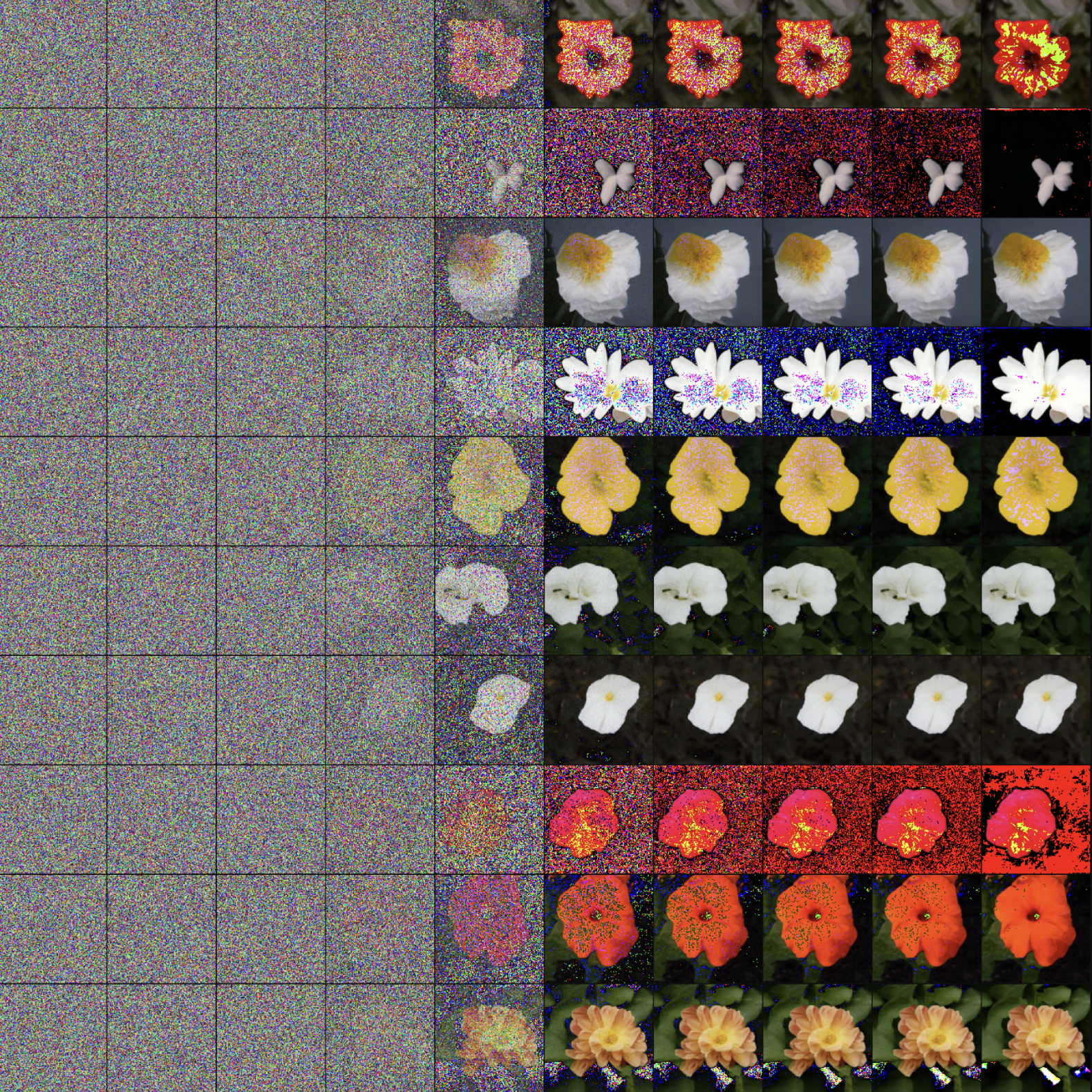
The function sample is sampling pure Gaussian noises at $t=T$ and then denoising it back to the original signal in a generative way.

6. Training

# Train Model using DataParallel
# Better way is to use DDP
device = "cuda:0" if torch.cuda.is_available() else "cpu"

noise2noise = UNet(dim=IMAGE_SIZE, channels=CHANNELS, dim_mults=(1, 2, 4), use_convnext=False)
print('Number of Parameters = ', sum(p.numel() for p in noise2noise.parameters() if p.requires_grad))

if torch.cuda.device_count() > 1:
    print("Using", torch.cuda.device_count(), "GPUs!")
    noise2noise = torch.nn.DataParallel(noise2noise)

noise2noise.to(device)
optimizer = Adam(noise2noise.parameters(), lr=1e-3)

# train on!!

dataloader = DataLoader(dataset['train'], collate_fn=collate_fn, batch_size=192)
print('dataloader length = ', len(dataloader))

# epochs need to be T * normal_epochs
# so that almost all the noisy images will get sampled
epochs = 1000

for epoch in tqdm(range(epochs)):
    
    for step, batch_images in enumerate(dataloader):
        
        optimizer.zero_grad()

        batch_size = batch_images.shape[0]
        batch_images = batch_images.to(device)

        # Algorithm 1 line 3: sample t uniformally for every example in the batch
        t = torch.randint(0, T, (batch_size, ), device=device, dtype=torch.long)

        loss = p_losses(noise2noise, batch_images, t, loss_type='L1')

        # if step % 100 == 0: print(f'Epoch: {epoch:02d} | Step: {step:03d} | Loss: {loss.item():.3f}')

        loss.backward()
        optimizer.step()
    
    if epoch % 5 == 0: print(f'Epoch: {epoch:02d} | Step: {step:03d} | Loss: {loss.item():.3f}')

now = datetime.now().strftime("%Y-%m-%d-%H-%M-%S")
model_name = f'Diffusion_Flower_{epochs}_{now}'
torch.save(noise2noise.state_dict(), os.path.join('/home/ubuntu/trained_models/', f'{model_name}.pt'))

Output:

Number of Parameters =  32009619
Using 8 GPUs!
dataloader length =  43

Epoch: 00 | Step: 042 | Loss: 0.801
Epoch: 05 | Step: 042 | Loss: 1.022
Epoch: 10 | Step: 042 | Loss: 0.416
Epoch: 15 | Step: 042 | Loss: 0.206
...
Epoch: 835 | Step: 042 | Loss: 0.065
Epoch: 840 | Step: 042 | Loss: 0.067

The DDPM model might also be quite memory expensive due to the IMAGE_SIZE and the Attention mechanism in the UNet (on top of the ResNet parameters..).

batch size > 24: memory explodes for 1 GPU

current speed = 240s / epoch @ batch_size = 24 on 1 GPU
current speed = 110s / epoch @ batch_size = 64 on 4 GPUs
current speed = 110s / epoch @ batch_size = 96 on 4 GPUs
current speed = 116s / epoch @ batch_size = 192 on 8 GPUs

7. Generating

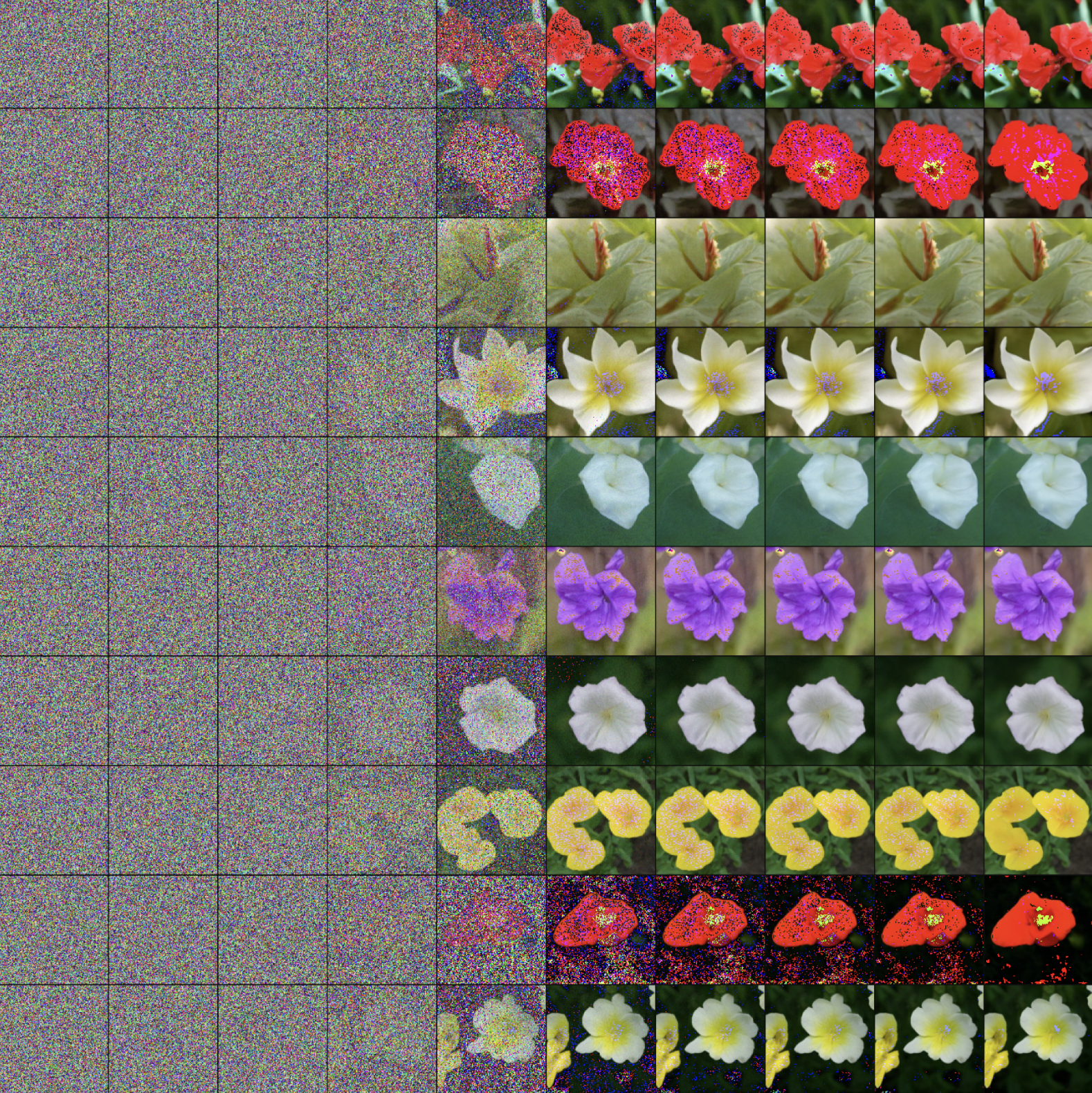
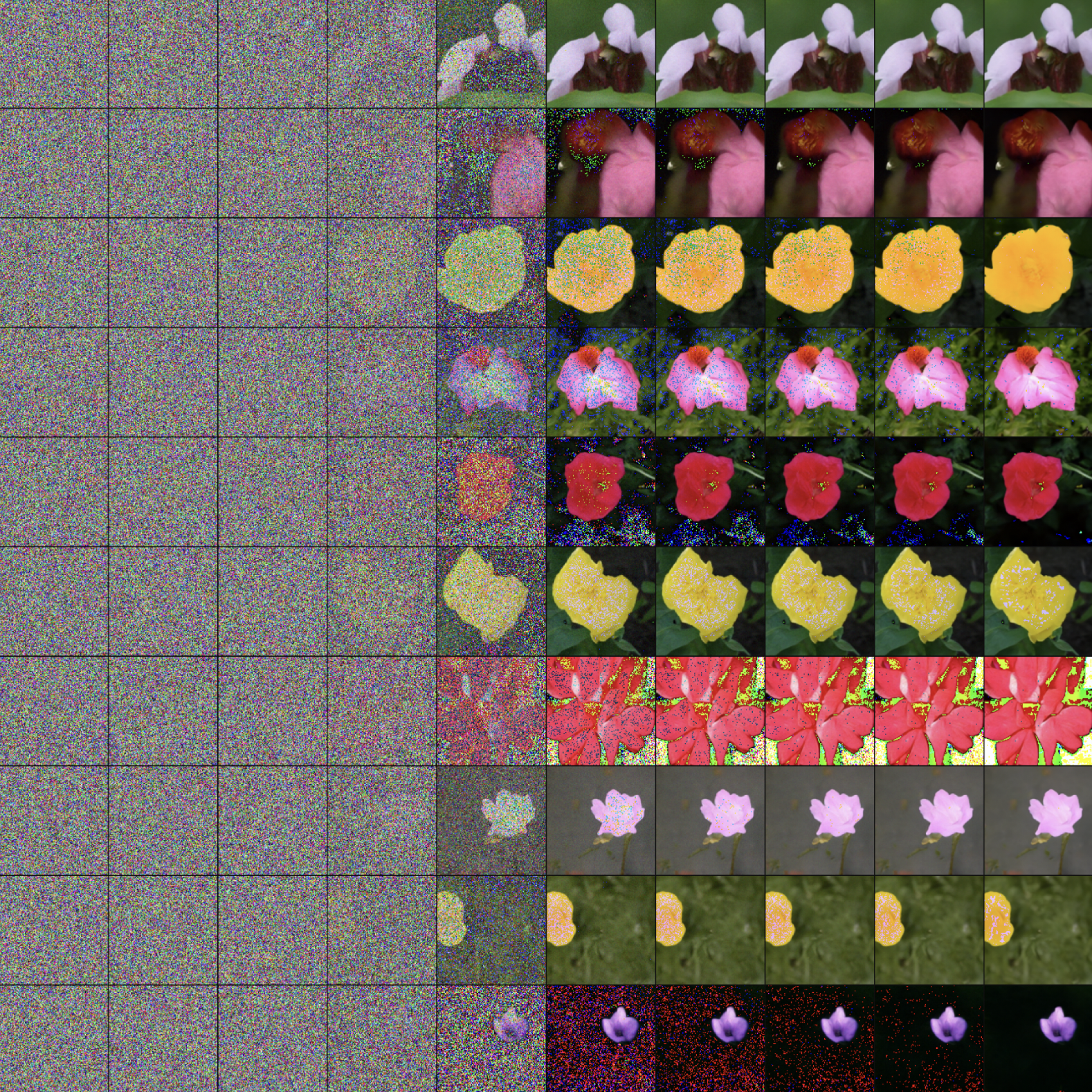
After the model got trained, it’ll be interesting to take a look at some of the generated images:

# sample 64 images
samples = sample(noise2noise, image_size=IMAGE_SIZE, batch_size=64, channels=CHANNELS)
ts = [0, 50, int(0.5 * T), int(0.75 * T), int(0.9 * T), T-10, T-5, T-3, T-2, T-1]
samples_for_plot = [[flower_reverse_transformation(torch.tensor(samples[j][6 * i, :, :, :])) for j in ts] for i in range(10)]
plot(samples_for_plot)

Output:

8. Notes

The generative power of DDPM is really strong and the model formulation is cool and with physics intuition behind it.

The Time Embedding dictates the UNet to be lowpass-like filter in the later time points ($t \sim T$), generating contours or global shapes from the noises. In the earlier time points ($t << T$), it performs like a highpass filter, denoising the high frequency noises away and resulting in a high resolution images that approximates the image distribution of the training data set. One can attenuate the denoising power, say, making it less stochastic by averaging 10 or more denoised images together at one step. It will make the image less hallucinated but also more blurry as one tries to averaging out some high-resolution signals that correspond to different end results. It is also the tradeoff between FID and IS in generative models

References

Jonathan Ho, Ajay Jain, Pieter Abbeel, Denoising Diffusion Probabilistic Models, https://arxiv.org/abs/2006.11239, 2020
Calvin Luo, Understanding Diffusion Models: A Unified Perspective, https://arxiv.org/abs/2208.11970, 2022
Ashish Vaswani, Noam Shazeer, Niki Parmar, Jakob Uszkoreit, Llion Jones, Aidan N. Gomez, Lukasz Kaiser, Illia Polosukhin, Attention Is All You Need, https://arxiv.org/abs/1706.03762, 2017
https://lilianweng.github.io/posts/2021-07-11-diffusion-models/
https://huggingface.co/blog/annotated-diffusion